Style Sampler
Layout Style
Patterns for Boxed Mode


Backgrounds for Boxed Mode
Search News Posts
General Inquiries 1-888-555-5555
•
Support 1-888-555-5555

Churn Detection
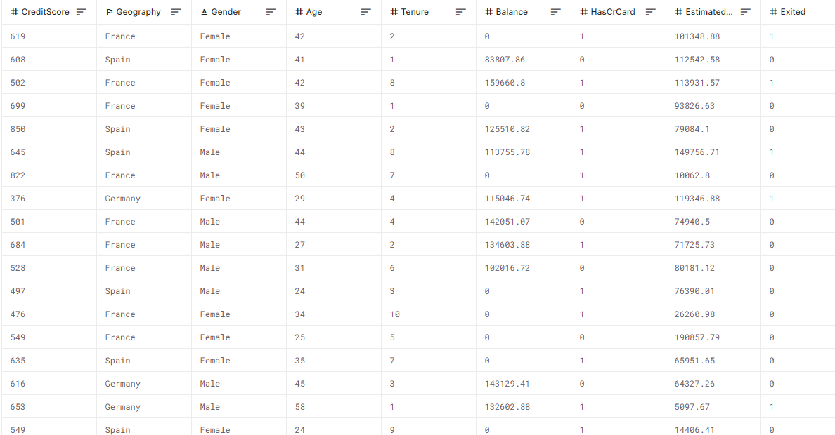
The dataset includes 14 features about the customers and their products at a bank along with 10,000 customers (i.e. rows). Using the features, the goal is to determine whether a customer will churn (exited = 1). We therefore want to create a supervised learning method to carry out a classification task using machine learning.
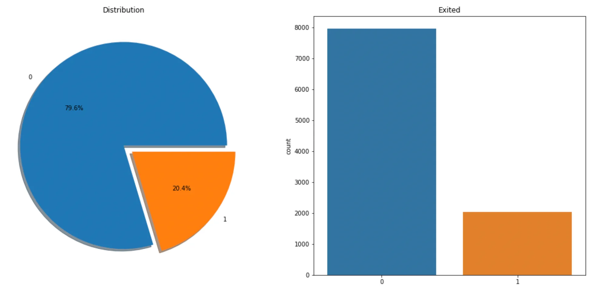
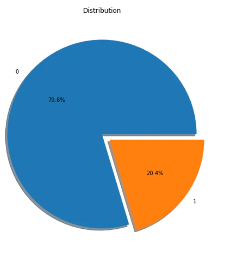
Churn prediction is likely to have an imbalance class distribution. The number of customers who churned (i.e. left) is usually much less than the number of customers who did not churn. We can check the distribution of values with the value_counts function. We see that there is imbalance in the target variable. There is an imbalance in the target variable (“Exited”). It is important to eliminate the imbalance.
Churn prediction is likely to have an imbalance class distribution. The number of customers who churned (i.e. left) is usually much less than the number of customers who did not churn. We can check the distribution of values with the value_counts function. We see that there is imbalance in the target variable. There is an imbalance in the target variable (“Exited”). It is important to eliminate the imbalance.
Churn prediction is likely to have an imbalance class distribution. The number of customers who churned (i.e. left) is usually much less than the number of customers who did not churn. We can check the distribution of values with the value_counts function. We see that there is imbalance in the target variable. There is an imbalance in the target variable (“Exited”). It is important to eliminate the imbalance.
The essential decision we need to make is how many units or Product X to produce each week. That's our decision variable which we denote as x. The weekly revenues are then $270x. The costs include the value of the raw materials and each form of labor. If we produce x units a week, then the total cost is $40x. which means there is a profit earned on each unit of X produced, so let's produce as many as possible.
There are three constraints that limit how many units can be produced. There is market demand for no more than 40 units per week. Producing x = 40 units per week will require 40 hours per week of Labor A, and 80 hours per week of Labor B. Checking those constraints we see that we have enough labor of each type, so the maximum profit will be $1600 per week. What we conclude is that market demand is the 'most constraining constraint.' Once we've made that deduction, the rest is a straightforward problem that can be solved by inspection.
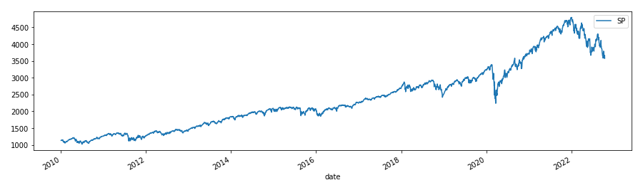
The graph below samples one such visualization that you would use to capture a trend hidden in the sample data set shared earlier on in the case study.
DATE
CAC
DAX
DJI
SP
FTSE
NIKKEI
NASDAQ
VIX
04.01.2010
4013,96
6048,29
10583,95
4013,96
6048,29
10583,95
4013,96
6048,29
05.01.2010
4013,96
6048,29
10583,95
4013,96
6048,29
10583,95
4013,96
6048,29
06.01.2010
4013,96
6048,29
10583,95
4013,96
6048,29
10583,95
4013,96
6048,29
07.01.2010
4013,96
6048,29
10583,95
4013,96
6048,29
10583,95
4013,96
6048,29
08.01.2010
4013,96
6048,29
10583,95
4013,96
6048,29
10583,95
4013,96
6048,29
...
...
...
...
...
...
...
...
...
08.01.2022
4013,96
6048,29
10583,95
4013,96
6048,29
10583,95
4013,96
6048,29
It shows the status of the S&P 500 stock index published by Standard & Poor's.
Click on Calculate Return button to see portfolio return results and maximum benefit.
SP
count 2943.000000
mean 2372.644913
std 977.094492
min 1022.580017
25% 1547.070007
50% 2109.409912
75% 2900.479980
max 4793.540039
Maximum Benefit : 1715.0
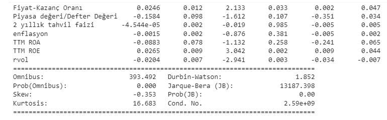
In this case study, Prediction modeling was done with Multivariate regression.
Click on the calculate button to see the portfolio return result!
Result:
As an example, downloading financial data from Yahoo Finance and investing.com via Python for company A is shown.
anaplatform Data Consultancy is a premium consulting company tailıred for businesses and corporations. anaplatform Data Consultancy is ideal for businesses of any type such as corporations, educational institutions, security firms and enterprise-level organizations.


