Style Sampler
Layout Style
Patterns for Boxed Mode


Backgrounds for Boxed Mode
Search News Posts
General Inquiries 1-888-555-5555
•
Support 1-888-555-5555

Demand Forecasting
In this study, daily and weekly demand forecasting results were compared for a chemical product company. The effect of the dollar exchange rate on demand was examined and the forecast for the next period was made over the period with the best results.
ChampionX, manufactures and distributes a wide array of chemical agents, products, parts, and exploitation tools to other manufacturers. In 2021, ChampionX reported a total revenue of 3B$ doing business in over 60 countries with 7,000 employees. Currently reviewing their inventory and forecasting practices, they have solicited our aid to increase their forecast accuracy while offering insights on the optimal aggregation level for forecasting demand.
We have decided to make the best use of both statistical-based and machine-learning-based models. Optimizing each to the best extent, to finally compare their accuracy and bias to select the best solution.
The dataset being erratic, we have chosen a simple combination of Median Absolute Error (MAE, or forecast error in the figures) and bias to assess the forecasting quality of our forecasts. This combination has the advantage of being simple to interpret while looking at accuracy and bias.
We identified product transitions throughout our intensive data-cleaning exercise. As illustrated in the figure below, when a new product replaces another one, our model can look at the historical sales of the former to the advantage of forecasting the new one.
The dataset being erratic, we have chosen a simple combination of Median Absolute Error (MAE, or forecast error in the figures) and bias to assess the forecasting quality of our forecasts. This combination has the advantage of being simple to interpret while looking at accuracy and bias.
The essential decision we need to make is how many units or Product X to produce each week. That's our decision variable which we denote as x. The weekly revenues are then $270x. The costs include the value of the raw materials and each form of labor. If we produce x units a week, then the total cost is $40x. which means there is a profit earned on each unit of X produced, so let's produce as many as possible.
There are three constraints that limit how many units can be produced. There is market demand for no more than 40 units per week. Producing x = 40 units per week will require 40 hours per week of Labor A, and 80 hours per week of Labor B. Checking those constraints we see that we have enough labor of each type, so the maximum profit will be $1600 per week. What we conclude is that market demand is the 'most constraining constraint.' Once we've made that deduction, the rest is a straightforward problem that can be solved by inspection.
At the aggregated level, machine learning provides a 19% FVA compared to the benchmark (8% of FVA for the statistical model)
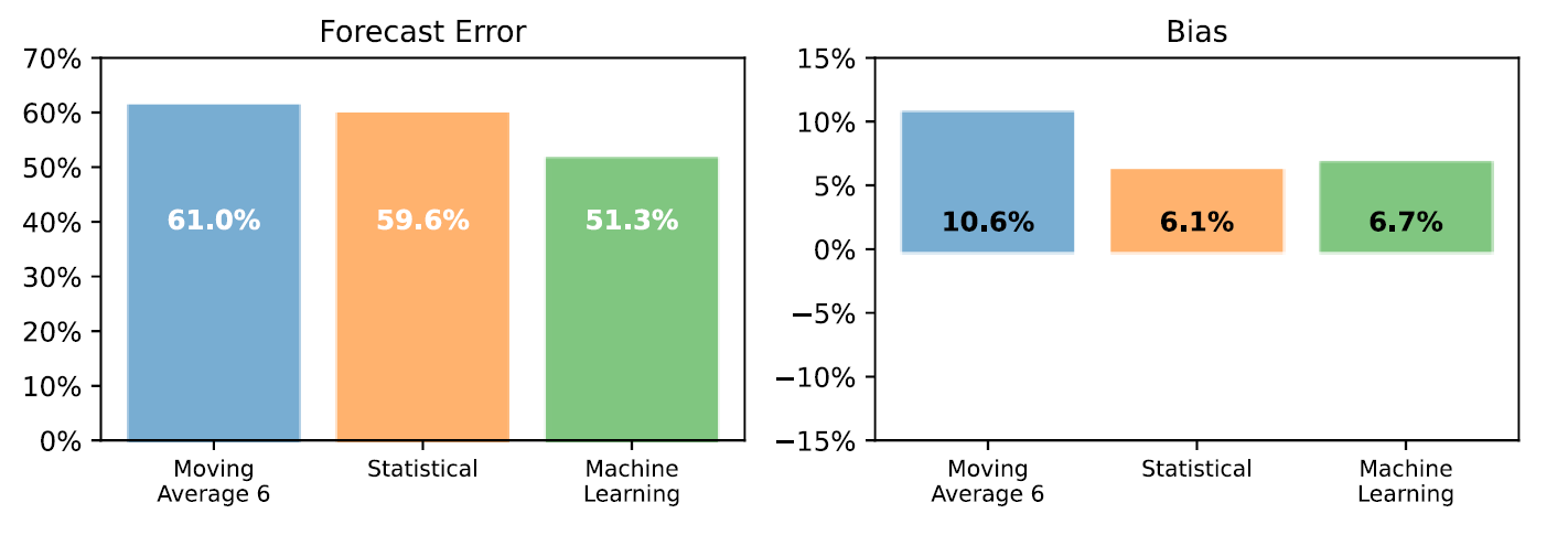
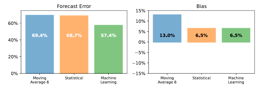
At the detailed level, machine learning provides a 22% FVA compared to the benchmark (9% of FVA for the statistical model).
As shown in the figure below, our machine-learning model delivered accurate forecasts over the 6-month horizon. The spread between the model and the benchmark even widens over time! Our model only loses around 1% accuracy per month, whereas the benchmark loses about 2%.
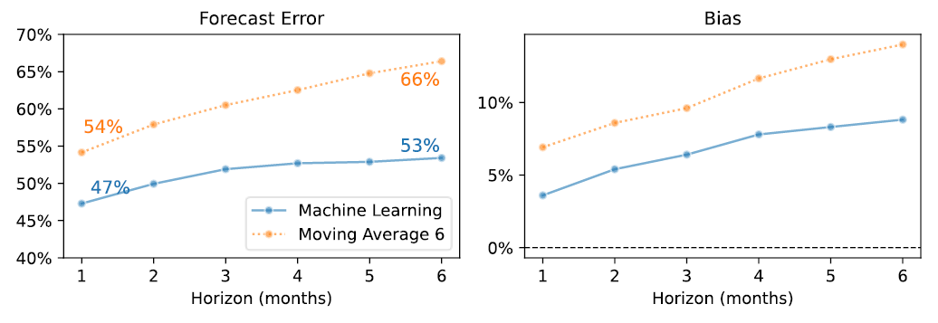
We used 6-month rolling-horizon forecasts (the first one with only 24 months of history!) to generate our second batch of tests. For our machine learning models, such a low amount of historical data is similar to fighting with one hand attached to your back. Nevertheless, it also successfully delivered 20% added value compared to the benchmark.
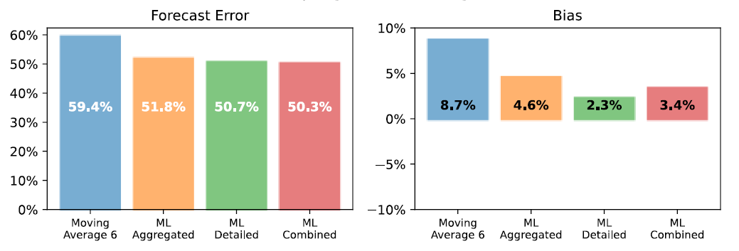
At the aggregated level, the combined forecast displays an FVA of 19.4% (1.6% short of the bottom-up forecast).
For multiple reasons, we do not recommend using external industry benchmarks when assessing forecasting accuracy. Instead, we compare our forecasting models against a moving average (and so should you!). In the past, simple naïve forecasts used to be considered suitable benchmarks. But they are too easy to beat. So instead, we look for the best moving average by trying out different horizons (3, 6, 12, and 24 months).
As displayed in the two figures above, the top-down forecast (made at a detailed level) provides slightly more accurate predictions than the bottom-up and combined forecasts.
Nevertheless, we decided to use the combined model as a final model. Indeed, we have good reasons to think that this combination will provide better, more insightful results over time than a single model top-down or bottom-up model.
Three weeks of work were needed to gather the correct pricing, product transitions and construct a clean dataset that could be fed into the various models. Two more weeks were spent creating the models and testing features and ideas. A final week was dedicated to analyzing the models’ performance and making the final report.
Let’s get in touch to see how much value advanced forecasting can deliver to your supply chain.
Anaplatform Data Consultancy is a premium consulting company tailored for businesses and corporations. anaplatform Data Consultancy is ideal for businesses of any type such as corporations, educational institutions, security firms and enterprise-level organizations.


